Contents

This is the webpage of XAEM version 0.1.1. The most updated version of XAEM is here:
https://www.meb.ki.se/sites/biostatwiki/xaem/

1. Introduction
2. Download and installation
3. XAEM: step by step instruction and explanation
3.1 Preparation for the annotation reference
3.2 Quantification of transcripts
4. A practical copy-paste example of running XAEM
5. Dataset for differential expression (DE) analysis

1. Introduction

This document shows how to use XAEM [Deng et al., 2019] to quantify isoform expression for multiple samples.

What are new in version 0.1.1

• Add standard error for the estimates
• Fix a small bug when separe a CRP into more than 1 CRP due to H_thres
• Fix a small bug in function crpcount() to avoid the error when having only 1 CRP

Older versions

• Code, data and instruction of most XAEM versions are available on the XAEM github site
• Webpage of XAEM version 0.1.0: click here to get there

Software requirements for XAEM:

• R version 3.3.0 or later with installed packages: foreach and doParallel
• C++11 compliant compiler (g++ >= 4.7)
• XAEM is currently tested in Linux OS environment

Annotation reference: XAEM requires a fasta file of transcript sequences and a gtf file of transcript annotation. XAEM supports all kinds of reference and annotation for any species. In the XAEM paper,  we use the UCSC hg19 annotation:

• Download the sequences of transcripts:transcripts.fa.gz
• Download the annotation of transcripts: genes_annotation.gtf.gz
• Download the design matrix X of this annotation:  X_matrix.RData (X matrix is an essential object for bias correction and isoform quantification, see Section 4.1.2 for more details)

wget https://www.meb.ki.se/sites/biostatwiki/wp-content/uploads/sites/4/XAEM_datasources/transcripts.fa.gz
gunzip transcripts.fa.gz
content/uploads/sites/4/XAEM_datasources/genes_annotation.gtf.gz
gunzip genes_annotation.gtf.gz
wget -O X_matrix.RData https://www.meb.ki.se/sites/biostatwiki/wp-content/uploads/sites/4/2022/09/X_matrix.rdata --no-check-certificate

2. Download and installation

If you use the binary version of XAEM (recommended):

• Download the latest binary version from XAEM website:

wget https://www.meb.ki.se/sites/biostatwiki/wp-content/uploads/sites/4/XAEM_datasources/XAEM-binary-0.1.1.tar.gz

• Uncompress to folder

tar -xzvf XAEM-binary-0.1.1.tar.gz

• Move to the XAEM_home directory and do the configuration for XAEM

cd XAEM-binary-0.1.1
bash configure.sh

• Add paths of lib folder and bin folder to LD_LIBRARY_PATH and PATH

export LD_LIBRARY_PATH=/path/to/XAEM-binary-0.1.1/lib:$LD_LIBRARY_PATH
export PATH=/path/to/XAEM-binary-0.1.1/bin:$PATH

If you want to build XAEM from sources:

• Download XAEM  and move to XAEM_home directory

wget https://www.meb.ki.se/sites/biostatwiki/wp-content/uploads/sites/4/2020/12/XAEM-source-0.1.1.tar_.gz
tar -xzvf XAEM-source-0.1.1.tar_.gz
cd XAEM-source-0.1.1
bash configure.sh

• XAEM requires information of flags from Sailfish including DFETCH_BOOST, DBOOST_ROOT, DTBB_INSTALL_DIR and DCMAKE_INSTALL_PREFIX. Please refer to the Sailfish website for more details of these flags.
• Do installation by the following command:

DBOOST_ROOT=/path/to/boostDir/ DTBB_INSTALL_DIR=/path/to/tbbDir/ DCMAKE_INSTALL_PREFIX=/path/to/expectedBuildDir bash install.sh

• After the installation is finished, remember to add the paths of lib folder and bin folder to LD_LIBRARY_PATH and PATH

export LD_LIBRARY_PATH=/path/to/expectedBuildDir/lib:$LD_LIBRARY_PATH
export PATH=/path/to/expectedBuildDir/bin:$PATH

Do not forget to replace “/path/to/” by your local path.

3. XAEM: step by step instruction and explanation

XAEM mainly contains the following steps:

• Preparation for the annotation reference:  to process the annotation of transcripts to get essential information for transcript quantification. This step includes 1) index transcript sequences and 2) Construct the design matrix X.
• Quantification of transcripts:  to get input from multiple RNA-seq samples to do quasi-mapping, generate data for quantifying transcript expression. This step consists of 1) generate equivalence class table; 2) create Y count matrix and 3) estimate transcript expression using AEM algorithm to update the X matrix and transcript (isoform) expression.

3.1 Preparation for the annotation reference

3.1.1 Indexing transcripts

Using TxIndexer to index the transcript sequences in the reference file (transcripts.fa). For example:

wget https://www.meb.ki.se/sites/biostatwiki/wp-content/uploads/sites/4/XAEM_datasources/transcripts.fa.gz
gunzip transcripts.fa.gz
TxIndexer -t /path/to/transcripts.fa -o /path/to/TxIndexer_idx

 3.1.2 Construction of the X matrix (design matrix)

This step constructs the X matrix required by the XAEM pipeline. For users working with human annotation of UCSC hg19  the X matrix can be downloaded here: X_matrix.rdata (need to rename the file to X_matrix.RData).

Given file transcripts.fa containing the transcript sequences of an annotation reference, we construct the design matrix as follows.

• a) Generate simulated RNA-seq data using the R-package “polyester”

## R-packages of "polyester" and "Biostrings" are required
Rscript XAEM_home/R/genPolyesterSimulation.R /path/to/transcripts.fa /path/to/design_matrix

• b) Run GenTC to generate Transcript Cluster (TC) using the simulated data. GenTC will generate an eqClass.txt file as the input for next step.

GenTC -i /path/to/TxIndexer_idx -l IU -1 /path/to/design_matrix/sample_01_1.fasta -2 /path/to/design_matrix/sample_01_2.fasta -p 8 -o /path/to/design_matrix

• c) Create a design matrix using buildCRP.R. The parameter setting for this function is as follows.
  • in: the input file (eqClass.txt) obtained from the last step.
  • out: the output file name (*.RData) which the design matrix will be saved.
  • H: (default H=0.025) is the threshold to filter false positive neighbors in each X matrix. (Please refer to the XAEM paper, Section 2.2.1)

Rscript XAEM_home/R/buildCRP.R in=/path/to/design_matrix/eqClass.txt out=/path/to/design_matrix/X_matrix.RData H=0.025

 3.2 Quantification of transcripts

Suppose we already created a working directory “XAEM_project” (/path/to/XAEM_project/) for quantification of transcripts.

 3.2.1 Generating the equivalence class table

The command to generate equivalence class table for each sample is similar to “sailfish quant”.  For example, we want to run XAEM for sample1 and sample2 with 4 cpus:

XAEM -i /path/to/TxIndexer_idx -l IU -1 s1_read1.fasta -2 s1_read2.fasta -p 4 -o /path/to/XAEM_project/sample1
XAEM -i /path/to/TxIndexer_idx -l IU -1 s2_read1.fasta -2 s2_read2.fasta -p 4 -o /path/to/XAEM_project/sample2

• If the data is compressed in gz format. We can combine with gunzip for a decompression on-fly:

XAEM -i /path/to/TxIndexer_idx -l IU -1 <(gunzip -c s1_read1.gz) -2 <(gunzip -c s1_read2.gz) -p 4 -o /path/to/XAEM_project/sample1
XAEM -i /path/to/TxIndexer_idx -l IU -1 <(gunzip -c s2_read1.gz) -2 <(gunzip -c s2_read2.gz) -p 4 -o /path/to/XAEM_project/sample2

3.2.2 Creating Y count matrix

After running XAEM there will be the output of the equivalence class table for multiple samples. We then create the Y count matrix. For example, if we want to run XAEM parallelly using 8 cores, the command is:

Rscript Create_count_matrix.R workdir=/path/to/XAEM_project core=8

3.2.3 Updating the X matrix and transcript expression using AEM algorithm

When finish the construction of Y count matrix, we use the AEM algorithm to update the X matrix. The updated X matrix is then used to estimate the transcript (isoform) expression. The command is as follows.

Rscript AEM_update_X_beta.R workdir=/path/to/XAEM_project core=8 design.matrix=X_matrix.RData isoform.out=XAEM_isoform_expression.RData paralog.out=XAEM_paralog_expression.RData merge.paralogs=FALSE isoform.method=average remove.ycount=TRUE

Parameter setting

• workdir: the path to working directory
• core: the number of cpu cores for parallel computing
• design.matrix: the path to the design matrix
• isoform.out (default=XAEM_isoform_expression.RData):  the output contains the estimated expression of individual transcripts, where the paralogs are split into separate isoforms. This file contains two objects: isoform_count and isoform_tpm for estimated counts and normalized values (TPM). The expression of the individual isoforms is calculated with the corresponding setting of parameter “isoform.method” below.
• isoform.method (default=average):  to report the expression of the individual members of a paralog as the average or total expression of the paralog set (value=average/total).
• paralog.out (default=XAEM_paralog_expression.RData): the output contains the estimated expression of merged paralogs. This file consists of two objects: XAEM_count and XAEM_tpm  for the estimated counts and normalized values (TPM). The standard error of the estimate is supplied in object XAEM_se stored in *.standard_error.RData.
• merge.paralogs (default=TRUE) (*): the parameter to turn on/off (value=TRUE/FALSE) the paralog merging in XAEM. Please see the details of how to use this parameter in the note at the end of this section.
• remove.ycount (default=TRUE): to clean all data of Ycount after use.

The output in this step will be saved in XAEM_isoform_expression.RData, which is the TPM value and raw read counts of multiple samples.

Note: (*) In XAEM pipeline we provide this parameter (merge.paralog) to merge or not merge the paralogs within the updated X matrix (please see XAEM paper Section 2.2.3 and Section 2.3).  Turning on (default) the paralog merging step produces a more accurate estimation. Turning off this step can produce the same sets of isoforms between different projects.

4. A practical copy-paste example of running XAEM

This section presents a tutorial to run XAEM pipeline with a toy example. Suppose that input data contain two RNA-seq samples and server supplies 4 CPUs for computation. We can test XAEM by just copy and paste of the example commands.

• Download the binary version of XAEM and do configuration

# Create a working folder
mkdir XAEM_example
cd XAEM_example
# Download the binary version of XAEM
wget https://www.meb.ki.se/sites/biostatwiki/wp-content/uploads/sites/4/XAEM_datasources/XAEM-binary-0.1.1.tar.gz

# Configure the tool
tar -xzvf XAEM-binary-0.1.1.tar.gz
cd XAEM-binary-0.1.1
bash configure.sh

# Add the paths to system
export LD_LIBRARY_PATH=$PWD/lib:$LD_LIBRARY_PATH
export PATH=$PWD/bin:$PATH
cd ..

• Download  annotation files and index the transcripts

## download annotation files
# Download the design matrix for the human UCSC hg19 annotation 
wget -O X_matrix.RData https://www.meb.ki.se/sites/biostatwiki/wp-content/uploads/sites/4/2022/09/X_matrix.rdata --no-check-certificate

# Download the fasta of transcripts in the human UCSC hg19 annotation 
wget https://www.meb.ki.se/sites/biostatwiki/wp-content/uploads/sites/4/XAEM_datasources/transcripts.fa.gz
gunzip transcripts.fa.gz

## Run XAEM indexer
TxIndexer -t transcripts.fa -o TxIndexer_idx

• Download the RNA-seq data of two samples: sample1 and sample2

## Download input RNA-seq samples
# Create a XAEM project to save the data
mkdir XAEM_project
cd XAEM_project

# Download the RNA-seq data
wget https://www.meb.ki.se/sites/biostatwiki/wp-content/uploads/sites/4/XAEM_datasources/sample1_read1.fasta.gz
wget https://www.meb.ki.se/sites/biostatwiki/wp-content/uploads/sites/4/XAEM_datasources/sample1_read2.fasta.gz
wget https://www.meb.ki.se/sites/biostatwiki/wp-content/uploads/sites/4/XAEM_datasources/sample2_read1.fasta.gz
wget https://www.meb.ki.se/sites/biostatwiki/wp-content/uploads/sites/4/XAEM_datasources/sample2_read2.fasta.gz
cd ..

• Generate the equivalence class tables for these samples

# Number of CPUs
CPUNUM=4

# Process for sample 1
XAEM -i TxIndexer_idx -l IU -1 <(gunzip -c XAEM_project/sample1_read1.fasta.gz) -2 <(gunzip -c XAEM_project/sample1_read2.fasta.gz) -p $CPUNUM -o XAEM_project/sample1

# Process for sample 2
XAEM -i TxIndexer_idx -l IU -1 <(gunzip -c XAEM_project/sample2_read1.fasta.gz) -2 <(gunzip -c XAEM_project/sample2_read2.fasta.gz) -p $CPUNUM -o XAEM_project/sample2

• Create Y count matrix

# Note: R packages "foreach" and "doParallel" are required for parallel computing
Rscript $PWD/XAEM-binary-0.1.1/R/Create_count_matrix.R workdir=$PWD/XAEM_project core=$CPUNUM design.matrix=$PWD/X_matrix.RData

• Estimate isoform expression using AEM algorithm

Rscript $PWD/XAEM-binary-0.1.1/R/AEM_update_X_beta.R workdir=$PWD/XAEM_project core=$CPUNUM design.matrix=$PWD/X_matrix.RData isoform.out=XAEM_isoform_expression.RData paralog.out=XAEM_paralog_expression.RData

The outputs are stored in the folder of “XAEM_project” including XAEM_isoform_expression.RData and XAEM_paralog_expression.RData.

5. Dataset for differential expression (DE) analysis

In XAEM paper we have used the RNA-seq data from the breast cancer cell line (MDA-MB-231) for DE analysis. Since the original data was generated by our collaborators and not published yet, we provide the equivalence class table by running the read-alignment tool Rapmap, which is the same mapper of Salmon and totally independent from XAEM algorithm. We also prepare the R scripts and the guide to replicate the DE analysis results in the paper.

In this section, we present an instruction to download the data and run the scripts. We try to build the pipeline following the copy-paste manner in shell, but the part of R scripts must be run in R console.

5.1 Download the R-scripts and the design matrix

This step is to download the R-scripts, change directory to the folder containing the R-scripts and download the design matrix.

# Download R-scripts
wget https://www.meb.ki.se/sites/biostatwiki/wp-content/uploads/sites/4/XAEM_datasources/brca_singlecell/RDR_brca_singlecell.zip
unzip RDR_brca_singlecell.zip
cd RDR_brca_singlecell

# Download the design matrix
wget -O X_matrix.RData https://www.meb.ki.se/sites/biostatwiki/wp-content/uploads/sites/4/2022/09/X_matrix.rdata --no-check-certificate

5.2 Run XAEM from the equivalence class tables which are the output of read-alignment tool Rapmap

Download the data of equivalence classes

# Download the table of equivalence classes of the single cells which are the output of read-alignment tool Rapmap

wget https://www.meb.ki.se/sites/biostatwiki/wp-content/uploads/sites/4/XAEM_datasources/brca_singlecell/brca_singlecell_eqclassDir.zip
unzip brca_singlecell_eqclassDir.zip

Run XAEM with the input from the equivalence class table using the R-codes below. Note:  This step takes about 2 hours using a personal computer with 4 CPUs. Users can consider skipping this step and downloading the available XAEM results for the downstream analysis.

# set the project path
projPath=getwd();
setwd(projPath)
source("collectDataOfXAEM.R")

If users want to download the available XAEM results

# Download the available results of XAEM

wget https://www.meb.ki.se/sites/biostatwiki/wp-content/uploads/sites/4/XAEM_datasources/brca_singlecell/XAEM_results.zip
unzip XAEM_results.zip

5.3 Differential-expression analysis of XAEM and other methods

Download the data of cufflinks and salmon. These files contain the read-count data of methods with and without using bias correction.

# Download the results of cufflinks
wget https://www.meb.ki.se/sites/biostatwiki/wp-content/uploads/sites/4/XAEM_datasources/brca_singlecell/cufflinks_results.zip
unzip cufflinks_results.zip

# Download the results of salmons
wget https://www.meb.ki.se/sites/biostatwiki/wp-content/uploads/sites/4/XAEM_datasources/brca_singlecell/salmon_results.zip
unzip salmon_results.zip

Run the codes below in R to do normalization and differential expression analysis.

# set the project path
projPath=getwd();
setwd(projPath)

# Normalize the data of three methods XAEM, Salmon and Cufflinks
source("Isoform_Expression_CPM_Normalization.R")

# Do DE analysis and plot figures
source("DEanalysis_plots.R")

# output: DE_Analysis.png

The results of the differential expression analysis (Figure 1 below) are the plots (DE_Analysis.png) reproducing Figure 3 of the XAEM paper. Note that due to the randomness of 50 times’ run, the figure might be slightly different from the figure in the paper.

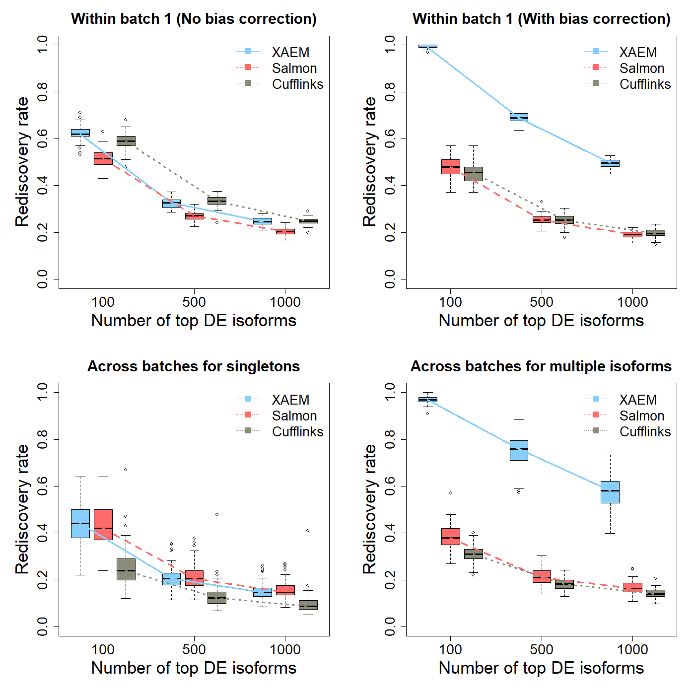
Figure 1. Detection and validation of differentially expressed (DE) isoforms using the MDA- MB-231 scRNA-seq dataset. XAEM, Salmon and Cufflinks are presented in blue-solid, red-dashed and grey-dotted lines, respectively. The x-axis shows the number of top DE isoforms in the training set; the y-axis is the proportion of rediscovery in the validation set. The rediscovery rate (RDR) is calculated by comparing the top 100, 500 and 1000 DE isoforms from the training set with all the significant DE isoforms from the validation set. The boxplots show the RDR from 50 times’ run. (a) Both training set and validation set are constructed using cells from batch 1. The quantification of XAEM, Salmon and Cufflinks is performed without bias correction. (b) The quantification from the three methods are bias- corrected. (c) The training set is constructed using cells from batch 1, while the validation set uses cells from batch 2. The RDR is calculated for only singleton isoforms. (d) The training set is constructed using cells from batch 1, and the validation set using cells from batch 2. The RDR is calculated using only non-paralogs.

References: 

1. Deng, Wenjiang, Tian Mou, Nifang Niu, Liewei Wang, Yudi Pawitan, and Trung Nghia Vu. 2019. “Alternating EM Algorithm for a Bilinear Model in Isoform Quantification from RNA-Seq Data.” Bioinformatics.  https://doi.org/10.1093/bioinformatics/btz640.

A fast and accurate methodology for discovery of circular RNAs from paired-end RNA-sequencing data

Contents

1. Introduction
2. Download and installation
3. Prepare BSJ reference database and annotation files
4. Indexing transcriptome and BSJ reference database
5. Run Circall pipeline
6. A practical copy-paste example of running Circall
7. Circall simulator

Update news

19 June 2020: version 0.1.0

• First submission

1. Introduction

Circall is a novel method for fast and accurate discovery of circular RNAs from paired-end RNA-sequencing data. The method controls false positives by two-dimensional local false discovery method and employs quasi-mapping for fast and accurate alignments. The details of Circall are described in its manuscript. In this page, we present the Circall tool and how to use it.

Software requirements:

Circall is implemented in R and C++. We acknowledge for materials from Sailfish, Rapmap and other tools used in this software.

• A C++-11 compliant compiler version of GCC (g++ >= 4.8.2)
• R packages version 3.6.0 or later with the following installed packages: GenomicFeatures, Biostrings, foreach, and doParallel.

Annotation reference

Circall requires

1. a fasta file of transcript sequences and a gtf file of transcript annotation: can be downloaded from public repositories such as Ensembl (ensembl.org)
2. a genome file of transcript sequences and a gtf file of transcript annotation: can be downloaded from public repositories such as Ensembl (ensembl.org)
3. an RData file of supporting annotation: A description of how to create the RData file for new annotation versions or species is available in the following Section.

The current Circall version was tested on the human genome, transcriptome with ensembl annotation version GRCh37.75. Specifically, the following files are required:

• Sequences of genome (ensembl website) GRCh37.75 genome fasta
• Sequences of transcripts (ensembl website) GRCh37.75 cdna fasta
• Gtf annotation of transcripts (ensembl website) GRCh37.75 gtf annotation

Versions

The latest version and information of Circall is updated at: https://www.meb.ki.se/sites/biostatwiki/circall/

2. Download and installation

If you use the binary verion of Circall:

• Download the latest binary version from Circall website

wget --no-check-certificate -O Circall_v0.1.0_linux_x86-64.tar.gz https://www.meb.ki.se/sites/biostatwiki/wp-content/uploads/sites/4/2021/04/Circall_v0.1.0_linux_x86-64.tar_.gz

• Uncompress to folder

tar -xzvf Circall_v0.1.0_linux_x86-64.tar.gz

• Move to the Circall_home directory and do configuration for Circall

cd Circall_v0.1.0_linux_x86-64
bash config.sh
cd ..

• Add paths of lib folder and bin folder to LD_LIBRARY_PATH and PATH

export LD_LIBRARY_PATH=/path/to/Circall_v0.1.0_linux_x86-64/linux/lib:$LD_LIBRARY_PATH
export PATH=/path/to/Circall_v0.1.0_linux_x86-64/linux/bin:$PATH

• Do not forget to replace “/path/to/” with your local path or use this command to automatically replace your path:

export LD_LIBRARY_PATH=$PWD/Circall_v0.1.0_linux_x86-64/linux/lib:$LD_LIBRARY_PATH
export PATH=$PWD/Circall_v0.1.0_linux_x86-64/linux/bin:$PATH

If you want to build Circall from sources:

• Download Circall from Circall website and move to Circall_home directory

wget --no-check-certificate -O Circall_v0.1.0.tar.gz https://www.meb.ki.se/sites/biostatwiki/wp-content/uploads/sites/4/2021/04/Circall_v0.1.0.tar_.gz
tar -xzvf Circall_v0.1.0.tar.gz
cd Circall_v0.1.0
bash config.sh

• Circall requires information of flags from Sailfish including DFETCH_BOOST, DBOOST_ROOT, DTBB_INSTALL_DIR and DCMAKE_INSTALL_PREFIX. Please refer to the Sailfish website for more details of these flags.
• Do installation by the following command:

DBOOST_ROOT=/path/to/boostDir/ DTBB_INSTALL_DIR=/path/to/tbbDir/ DCMAKE_INSTALL_PREFIX=/path/to/Circall_home bash install.sh

-After the installation is finished, remember to add the paths of lib folder and bin folder to LD_LIBRARY_PATH and PATH

export LD_LIBRARY_PATH=/path/to/Circall_home/lib:$LD_LIBRARY_PATH
export PATH=/path/to/Circall_home/bin:$PATH

Install Circall from sources in Ubuntu

##########################
### This contain scripts in the copy-and-paste manner (line-by-line) to install Circall from source codes
### The scripts have been successfully tested in Ubuntu 16, 19 and 20.

##########################
### download Circall
wget wget --no-check-certificate -O Circall_v0.1.0.tar.gz https://www.meb.ki.se/sites/biostatwiki/wp-content/uploads/sites/4/2021/04/Circall_v0.1.0.tar_.gz
tar -xzvf Circall_v0.1.0.tar.gz
cd Circall_v0.1.0

#config to run Circall
bash config.sh

### install boost_1_55_0
wget http://sourceforge.net/projects/boost/files/boost/1.58.0/boost_1_58_0.tar.gz
tar -xvzf boost_1_58_0.tar.gz
cd boost_1_58_0

sudo apt-get update
sudo apt-get install build-essential g++ python-dev autotools-dev libicu-dev build-essential libbz2-dev libboost-all-dev
sudo apt-get install aptitude
aptitude search boost

./bootstrap.sh --prefix=boost_1_58_0_build
./b2
./b2 install

#The Boost C++ Libraries were successfully built!
#add the lib and folder to paths
export LD_LIBRARY_PATH=$PWD/boost_1_58_0_build/stage/lib:$LD_LIBRARY_PATH
export PATH=$PWD/boost_1_58_0_build:$PATH


### install tbb44_20160526oss
cd ..
wget https://www.threadingbuildingblocks.org/sites/default/files/software_releases/source/tbb44_20160526oss_src_0.tgz
tar xvf tbb44_20160526oss_src_0.tgz
sudo apt-get install libtbb-dev

### install cmake for ubuntu: cmake 3.5.1
sudo apt install cmake
### install curl
sudo apt install curl
### install autoconf
sudo apt-get install autoconf
### install zlib
sudo apt install zlib1g-dev
sudo apt install zlib1g
### update all installations
sudo apt-get update

### install Circall
DBOOST_ROOT=$PWD/boost_1_58_0/boost_1_58_0_build/ DTBB_INSTALL_DIR=$PWD/tbb44_20160526oss/ DCMAKE_INSTALL_PREFIX=Circall_0.1.0_build bash install.sh

#The Circall_0.1.0 was successfully built!
###########

#add lib and bin folders to paths
export LD_LIBRARY_PATH=$PWD/Circall_0.1.0_build/lib:$LD_LIBRARY_PATH
export PATH=$PWD/Circall_0.1.0_build/bin:$PATH

#done
###########

3. Prepare BSJ reference database and annotation files

Download genome fasta, transcript fasta and gtf annotation files.

wget http://ftp.ensembl.org/pub/release-75/fasta/homo_sapiens/dna/Homo_sapiens.GRCh37.75.dna.primary_assembly.fa.gz
gunzip Homo_sapiens.GRCh37.75.dna.primary_assembly.fa.gz
wget http://ftp.ensembl.org/pub/release-75/fasta/homo_sapiens/cdna/Homo_sapiens.GRCh37.75.cdna.all.fa.gz
gunzip Homo_sapiens.GRCh37.75.cdna.all.fa.gz
wget http://ftp.ensembl.org/pub/release-75/gtf/homo_sapiens/Homo_sapiens.GRCh37.75.gtf.gz
gunzip Homo_sapiens.GRCh37.75.gtf.gz

Create sqlite

Rscript Circall_v0.1.0_linux_x86-64/R/createSqlite.R Homo_sapiens.GRCh37.75.gtf Homo_sapiens.GRCh37.75.sqlite

Create BSJ reference database

The BSJ reference database for Homo_sapiens.GRCh37.75 was generated and able to download from Homo_sapiens.GRCh37.75_BSJ_sequences.fa. This file was generated by the following command:

Rscript Circall_v0.1.0_linux_x86-64/R/buildBSJdb.R gtfSqlite=Homo_sapiens.GRCh37.75.sqlite genomeFastaFile=Homo_sapiens.GRCh37.75.dna.primary_assembly.fa bsjDist=250 maxReadLen=150 output=Homo_sapiens.GRCh37.75_BSJ_sequences.fa

4. Indexing transcriptome and BSJ reference database

Index transcriptome

Circall_v0.1.0_linux_x86-64/linux/bin/TxIndexer -t Homo_sapiens.GRCh37.75.cdna.all.fa -o IndexTranscriptome

Index BSJ reference database

Circall_v0.1.0_linux_x86-64/linux/bin/TxIndexer -t Homo_sapiens.GRCh37.75_BSJ_sequences.fa -o IndexBSJ

Now, all annotation data are generated and ready to run Circall.

5. Run Circall pipeline

Suppose sample_01_1.fasta and sample_01_2.fasta are the input fastq files. For convenience, we prepared a toy example to test the pipeline, which can be downloaded here:

wget https://www.meb.ki.se/sites/biostatwiki/wp-content/uploads/sites/4/2021/07/sample_01_1.fasta_.gz
wget https://www.meb.ki.se/sites/biostatwiki/wp-content/uploads/sites/4/2021/07/sample_01_2.fasta_.gz

Circall can be run in one command wrapped in a bash script:

bash Circall_v0.1.0_linux_x86-64/Circall.sh -genome Homo_sapiens.GRCh37.75.dna.primary_assembly.fa -gtfSqlite Homo_sapiens.GRCh37.75.sqlite -txFasta Homo_sapiens.GRCh37.75.cdna.all.fa -txIdx IndexTranscriptome -bsjIdx IndexBSJ -dep Circall_v0.1.0_linux_x86-64/Data/Circall_depdata_human.RData -read1 sample_01_1.fasta.gz -read2 sample_01_2.fasta.gz -p 4 -tag testing_sample -c FALSE -o Testing_out

Inputs and parameters

Annotation data:

• genome — genome in fasta format
• gtfSqlite — genome annotation in Sqlite format
• txFasta — transcripts (cDNA) in fasta format
• txIdx — quasi-index of txFasta
• bsjIdx — quasi-index of BSJ reference fasta file

Input data:

• read1 — input read1: should be in gz format
• read2 — input read2: should be in gz format

Other parameters:

• dep — data contain depleted circRNAs: to specify the null data (depleted circRNA) for the two-dimensional local false discovery rate method. For convenience, we collect the null data from three human cell lines datasets Hela, Hs68, and Hek293 and provided in the tool: Circall_v0.1.0_linux_x86-64/Data/Circall_depdata_human.RData
• p — the number of threads: Default is 4
• tag — tag name of results: Default is “Sample”
• td — generation of tandem sequences: TRUE/FALSE value, default is TRUE
• c — clean intermediate data: TRUE/FALSE value, default is TRUE
• o — output folder: Default is the current directory

Output

The main output of Circall is provided in *_Circall_final.txt. In this file, each row indicates one circular RNA, and the information of one circular RNA is presented in 8 columns:

• chr: chromosome
• start: start position
• end: end position
• geneID: gene name that the circRNA belongs to
• circID: the ID of circRNA in the format “chr__start__end”
• junction_fragment_count: the number of fragment counts supporting the back-splicing-junction (BSJ)
• median_circlen: the median length of the circular RNA
• fdr: the false discovery rate computed from the two-dimensional local false discovery method

6. A practical copy-paste example of running Circall

In this section, we provide a practical example of using Circall in a copy-paste manner for a Hs68 cell line dataset.

Download and install Circall

wget --no-check-certificate -O Circall_v0.1.0_linux_x86-64.tar.gz https://www.meb.ki.se/sites/biostatwiki/wp-content/uploads/sites/4/2021/04/Circall_v0.1.0_linux_x86-64.tar_.gz

• Uncompress to folder

tar -xzvf Circall_v0.1.0_linux_x86-64.tar.gz

• Move to the Circall_home directory and do configuration for Circall

cd Circall_v0.1.0_linux_x86-64
bash config.sh
cd ..

• Add paths of lib folder and bin folder to LD_LIBRARY_PATH and PATH

export LD_LIBRARY_PATH=$PWD/Circall_v0.1.0_linux_x86-64/linux/lib:$LD_LIBRARY_PATH
export PATH=$PWD/Circall_v0.1.0_linux_x86-64/linux/bin:$PATH

Download genome fasta, transcript fasta and BSJ databases and annotation file.

# genome from ENSEMBL website
wget http://ftp.ensembl.org/pub/release-75/fasta/homo_sapiens/dna/Homo_sapiens.GRCh37.75.dna.primary_assembly.fa.gz
gunzip Homo_sapiens.GRCh37.75.dna.primary_assembly.fa.gz

# cDNA (transcript) and Gene annotation (gft) from ENSEMBL website
wget http://ftp.ensembl.org/pub/release-75/fasta/homo_sapiens/cdna/Homo_sapiens.GRCh37.75.cdna.all.fa.gz
gunzip Homo_sapiens.GRCh37.75.cdna.all.fa.gz
wget http://ftp.ensembl.org/pub/release-75/gtf/homo_sapiens/Homo_sapiens.GRCh37.75.gtf.gz
gunzip Homo_sapiens.GRCh37.75.gtf.gz

# pre-built BSJ databases from Circall website
wget https://www.meb.ki.se/sites/biostatwiki/wp-content/uploads/sites/4/files/circall/Homo_sapiens.GRCh37.75_BSJ_sequences.fa.gz
gunzip Homo_sapiens.GRCh37.75_BSJ_sequences.fa.gz

# Genarate Sqlite annotation
Rscript Circall_v0.1.0_linux_x86-64/R/createSqlite.R Homo_sapiens.GRCh37.75.gtf Homo_sapiens.GRCh37.75.sqlite

Index transcriptome

Circall_v0.1.0_linux_x86-64/linux/bin/TxIndexer -t Homo_sapiens.GRCh37.75.cdna.all.fa -o IndexTranscriptome

Index BSJ reference database

Circall_v0.1.0_linux_x86-64/linux/bin/TxIndexer -t Homo_sapiens.GRCh37.75_BSJ_sequences.fa -o IndexBSJ

Download Hs68 cell line RNA-seq data

wget ftp://ftp.sra.ebi.ac.uk/vol1/fastq/SRR444/SRR444975/SRR444975_1.fastq.gz
wget ftp://ftp.sra.ebi.ac.uk/vol1/fastq/SRR444/SRR444975/SRR444975_2.fastq.gz

Run Circall

bash Circall_v0.1.0_linux_x86-64/Circall.sh -genome Homo_sapiens.GRCh37.75.dna.primary_assembly.fa -gtfSqlite Homo_sapiens.GRCh37.75.sqlite -txFasta Homo_sapiens.GRCh37.75.cdna.all.fa -txIdx IndexTranscriptome -bsjIdx IndexBSJ -dep Circall_v0.1.0_linux_x86-64/Data/Circall_depdata_human.RData -read1 SRR444975_1.fastq.gz -read2 SRR444975_2.fastq.gz -p 4 -tag testing_sample -o SRR444975

7.  Circall simulator

Introduction

Circall simulator is a tool integrated in Circall to generate RNA-seq data of both circRNA and tandem RNA. The source codes are provided in R/Circall_simulator.R of the Circall tool. The main function of the simulator is Circall_simulator() which is able to be run in R console. This function requires the following parameters:

Parameter setting:

• circInfo: a data frame that contains 6 columns which are: Chr, start_EXONSTART, end_EXONEND, GENEID, cCount and FPKM. Chr is chromosome name with formated as 1:22, X, Y, Mt. start_EXONSTART is starting position starting exon of circRNA, end_EXONEND is ending position ending exon of circRNA, GENEID is gene ID contains circRNA (used to get gene model), cCount are number of read pair want to generate for the target circRNA and FPKM are Fragments Per Kilobase of transcript per Million of target circRNAs. This is used to simulate circular RNAs
• tandemInfo: a data frame similar to circInfo to simulate tandem RNAs. tandemInfo=NULL (the default value) to not simulate tandem RNAs
• error_rate: sequencing error rate, the default value is 0.005
• set.seed: set seed for reproducibility, the default value is 2018
• gtfSqlite: path to your annotation file, Sqlite formated (generated by GenomicFeatures)
• genomeFastaFile: path to your genome fasta file
• txFastaFile: path to your transcript fasta file (cDNA)
• out_name: prefix output folders, the default value is “Circall_simuation”
• out_dir: the directory contains output, the default value is the current directory
• lib_size: expected library size used when useFPKM=TRUE, the default value is NULL
• useFPKM boolean value to use FPKM or not, the default value is FALSE. When this useFPKM=TRUE, users need to set value for lib_size, and the simulator will use the abundance in column FPKM of circInfo/tandemInfo for simulation

A toy example for using Circall simulator

For an illustration of using Circall simulator, we provide in this section a toy example. Suppose your current working directory contains the installed Circall and the annotation data. First, we need to load the functions of the simulator into your R console:

source("Circall_v0.1.0_linux_x86-64/R/Circall_simulator.R")

Then we create objects circInfo and tandemInfo containing the information of CircRNAs and tandem RNAs

Chr = c(7,7,3,5,17,4,7,1,3,1,17,12,14,10,18,17,5,20,16,17)

start_EXONSTART = c(131113792,99795401,172363413,179296769,36918664,151509200,2188787,51906019,57832924,225239153,76187051,111923075,104490906,101556854,196637,21075331,74981032,60712420,56903641,80730328)

end_EXONEND = c(131128461,99796580,172365904,179315312,36918758,151509336,2270359,51913807,57882659,225528403,76201599,111924628,104493276,101572901,199316,21087123,74998635,60716000,56904648,80772810)

GENEID = c("ENSG00000128585","ENSG00000066923","ENSG00000144959","ENSG00000197226","ENSG00000108294","ENSG00000198589","ENSG00000002822","ENSG00000085832","ENSG00000163681","ENSG00000185842","ENSG00000183077","ENSG00000204842","ENSG00000156414","ENSG00000023839","ENSG00000101557","ENSG00000109016","ENSG00000152359","ENSG00000101182","ENSG00000070915","ENSG00000141556")

set.seed(2021)
cCount = sample(2:2000,20)
FPKM = rep(0,20)

BSJ_info = data.frame(Chr = Chr, start_EXONSTART = start_EXONSTART, end_EXONEND = end_EXONEND, GENEID = GENEID, cCount = cCount, FPKM = FPKM)

circSet=c(1:15)
circInfo = BSJ_info[circSet,]
tandemInfo = BSJ_info[-circSet,]

Finally, we run the simulator:

simulation = Circall_simulator(circInfo = circInfo, tandemInfo = tandemInfo, useFPKM=FALSE, out_name = "Tutorial", gtfSqlite = "Homo_sapiens.GRCh37.75.sqlite", genomeFastaFile = "Homo_sapiens.GRCh37.75.dna.primary_assembly.fa", txFastaFile = "Homo_sapiens.GRCh37.75.cdna.all.fa", out_dir= "./simulation_test")

You can find in the “./simulation_test” that contains the outputs including:

• simulation_setting: setting information of simulation of both circRNAs and tandem RNAs.
• circRNA_data: RNA seq data of CircRNAs
• tandem_data: RNA seq data of tandem RNA
• fasta sequences of tandem RNAs
• fasta sequences of circular RNAs

8. License

Circall uses GNU General Public License GPL-3.